2. Quick Start
This chapter will introduce how to control the robot to quickly start welding work using an actual welding project as an example (it is necessary to first obtain authorization for the welding plugin). Figure 2-1 and Figure 2-2 illustrate the welding preparations, where Figure 2-1 shows the workpiece to be welded, and Figure 2-2 shows the robot and the workpiece.
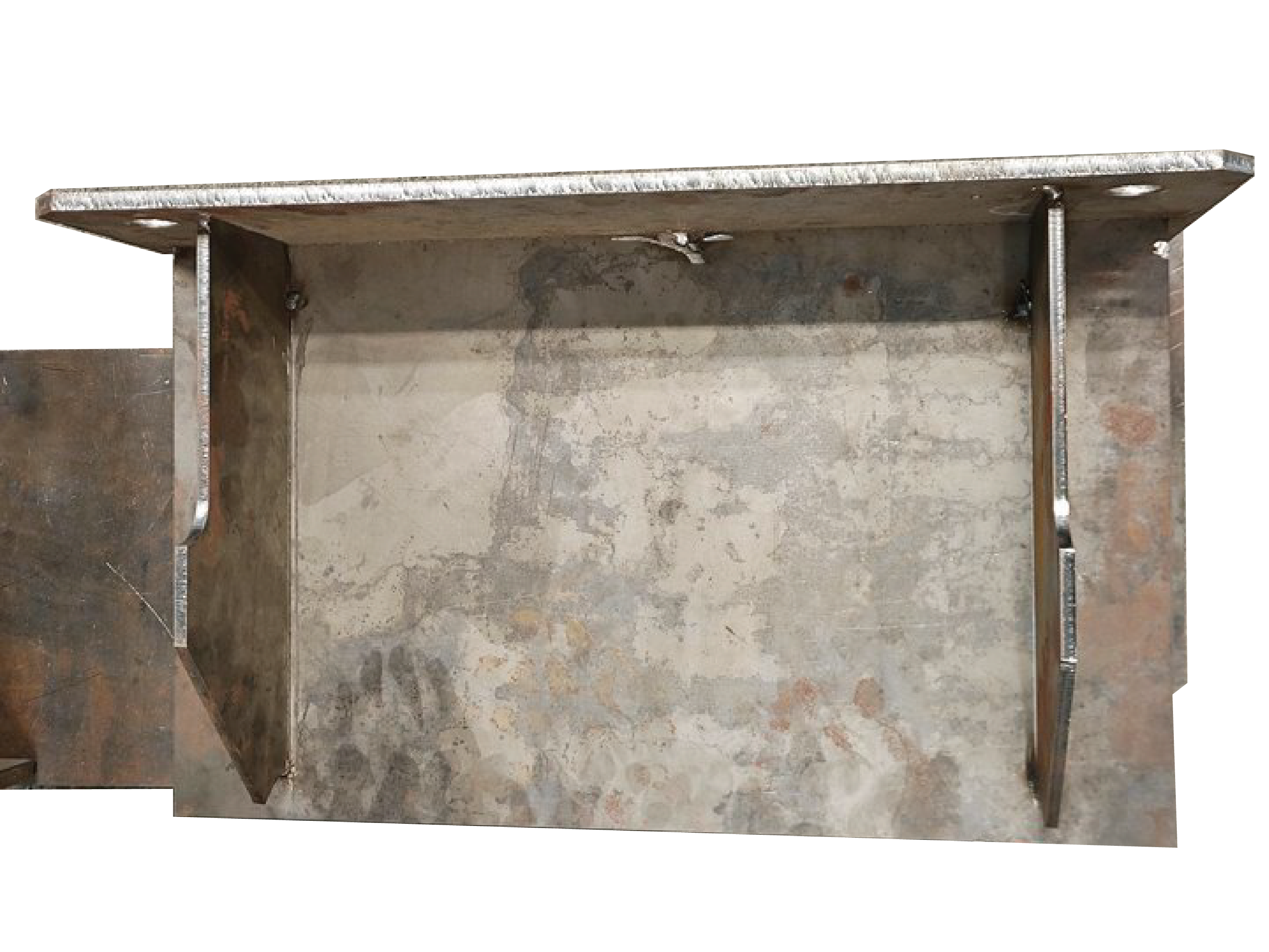
Figure 2.1 Workpiece to be Welded
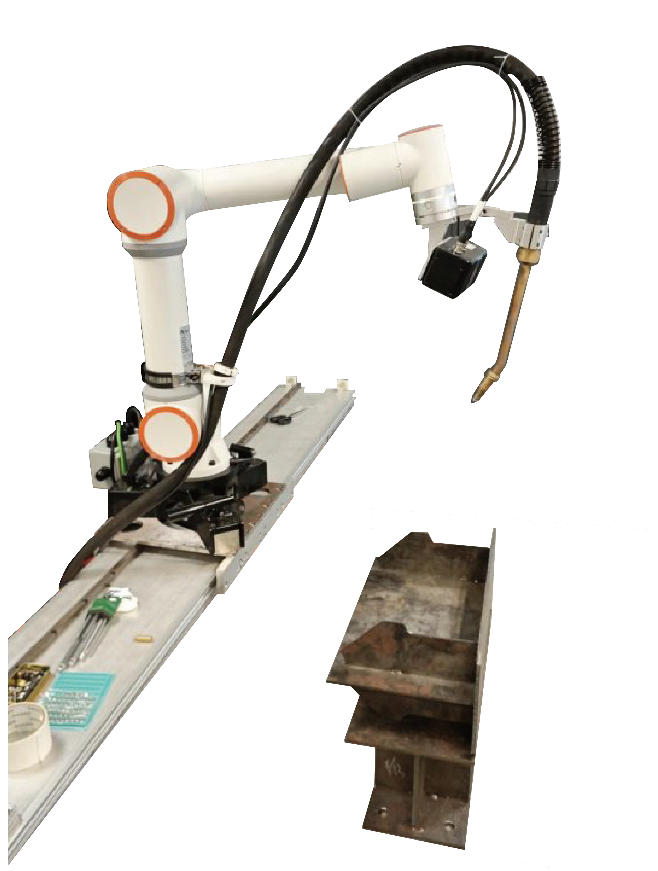
Figure 2.2 Robot + Workpiece
2.1. 3D MVC Product Description
This High-Precision 3D Camera utilizes grating-structured light projection and binocular stereo vision algorithms to reconstruct high-fidelity 3D point cloud data of objects, meeting industrial-grade requirements for high resolution and submillimeter measurement accuracy. Compact in size yet featuring a large depth of field and exceptional measurement precision, the system is designed for applications in industrial automation, robotics, and 3D object reconstruction.
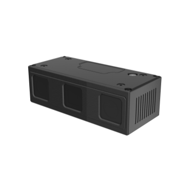
Figure 2.3 Standard version
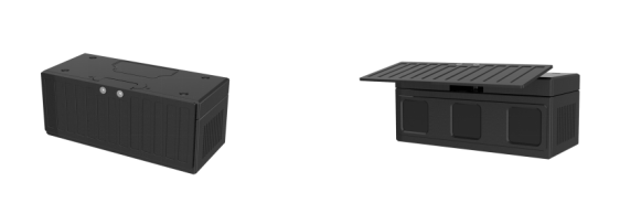
Figure 2.4 Version with protective cover
Key Features:
Welding Robot Integration: Compatible with mainstream welding robots for complex weld seam feature extraction, trajectory guidance, and workpiece alignment.
Advanced Imaging Algorithm: Achieves 0.2mm repeatability in Z-axis; employs binocular structured light technology for submillimeter-accurate image acquisition.
Multi-Frame Fusion: Mitigates reflections on metallic surfaces for reliable data.
Optimized Projection Module: Combines high-efficiency projection with precise exposure control for stable performance.
Robust Anti-Noise Capability: Delivers clear point clouds even for low-reflectivity or dark surfaces.
Non-Contact Measurement: Ensures zero damage to target objects.
Pre-Calibrated & Plug-and-Play: Factory-optimized settings eliminate user-side calibration.
Industrial-Grade Design:Fully enclosed aluminum alloy housing for durability;multi-mounting holes for flexible deployment.
Technical Specifications:
Working Distance: 350mm~1100mm.
Compact & Lightweight: High-strength body for easy integration.
High-Speed Imaging: Optimized for high-temperature environments (spark-resistant front cover included).
No-Teach Welding Path Generation: Enables autonomous operation without pre-programming.
2.1.1. System Requirements
OS: Windows 10.0 or later / Ubuntu 18.04 or later
CPU: 1.8GHz base clock or higher
RAM: 8GB or more (recommended)
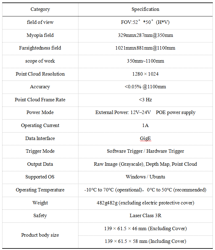
2.1.2. Product parameters
Table 2-1 Product Parameters
2.1.3. Field of view measurement range
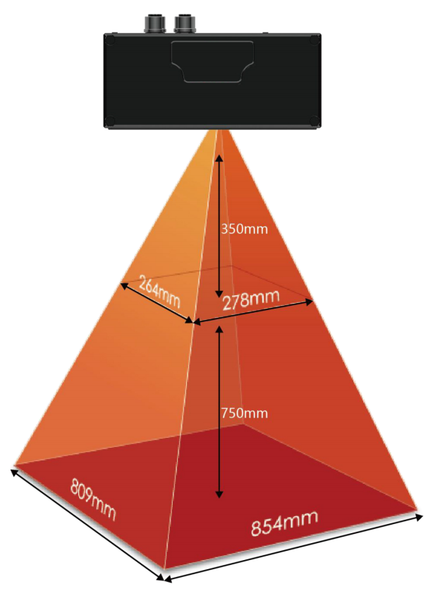
Figure 2.5 Field of view measurement range
2.1.4. Structural drawings
Standard version:
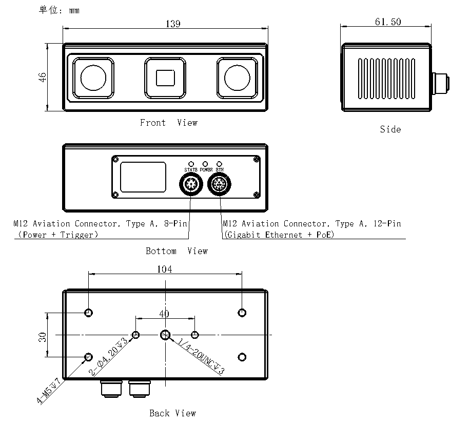
Figure 2.6 Standard version structural dimensions
Version with protective cover (optional):
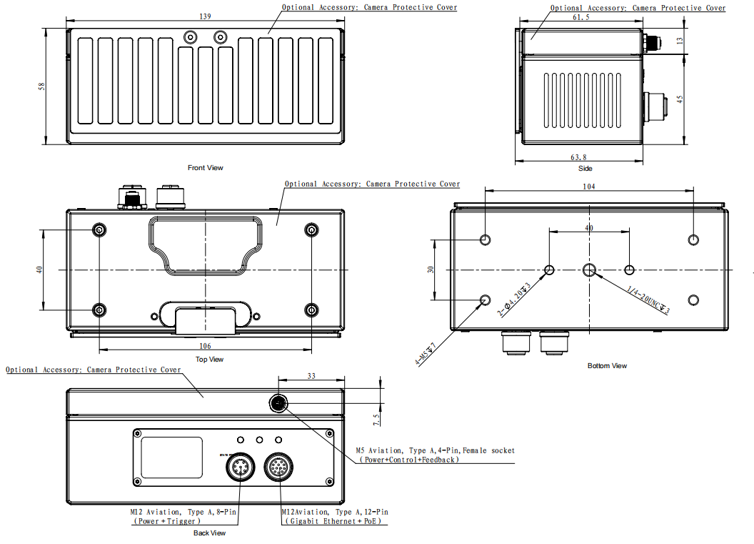
Figure 2.7 Version with protective cover (optional) structural dimensions
2.1.5. Communication interface
Camera power interface
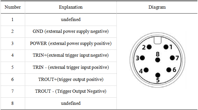
Body power socket (8pin)
Table 2-2 Power socket on the body (8pin)
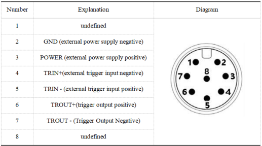
8-pin power cable
Table 2-3 Power cable (8pin)
Camera communication control interface
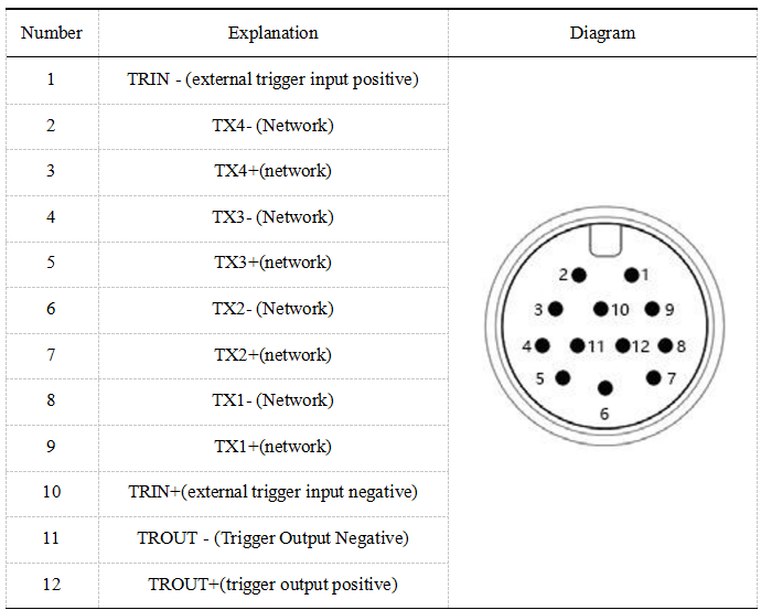
POE Ethernet port socket on the body (12pin)
Table 2-4 POE network port on the body (12pin)
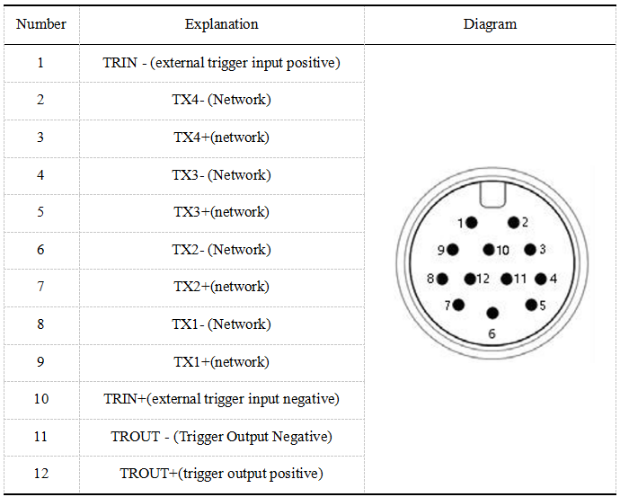
POE Ethernet cable (12pin)
Table 2-5 POE network cable (12pin)
Camera protective cover external control interface
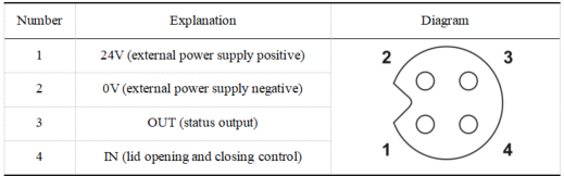
Protective cover outer control seat (4pin)
Table 2-6 Protective cover external control seat (4pin)
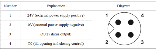
Protective cover external control cable (4pin)
Table 2-7 Protective cover external control cable (4pin)
2.1.6. Camera installation
Protective cover installation:
Remove the M5 plug from the camera’s upper housing to expose the cable entry port.
Secure the cover using four M3×12 hex socket head cap screws, aligning them with the corresponding mounting holes on the camera housing.
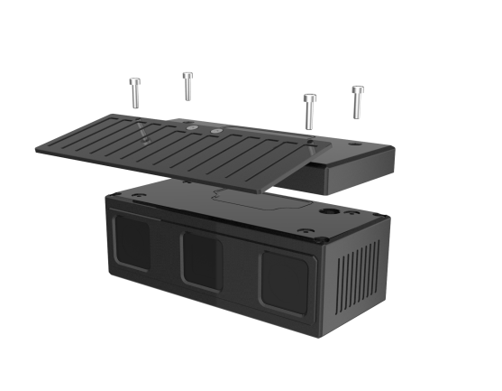
Figure 2.8 Protective cover installation diagram
Camera installation instructions:
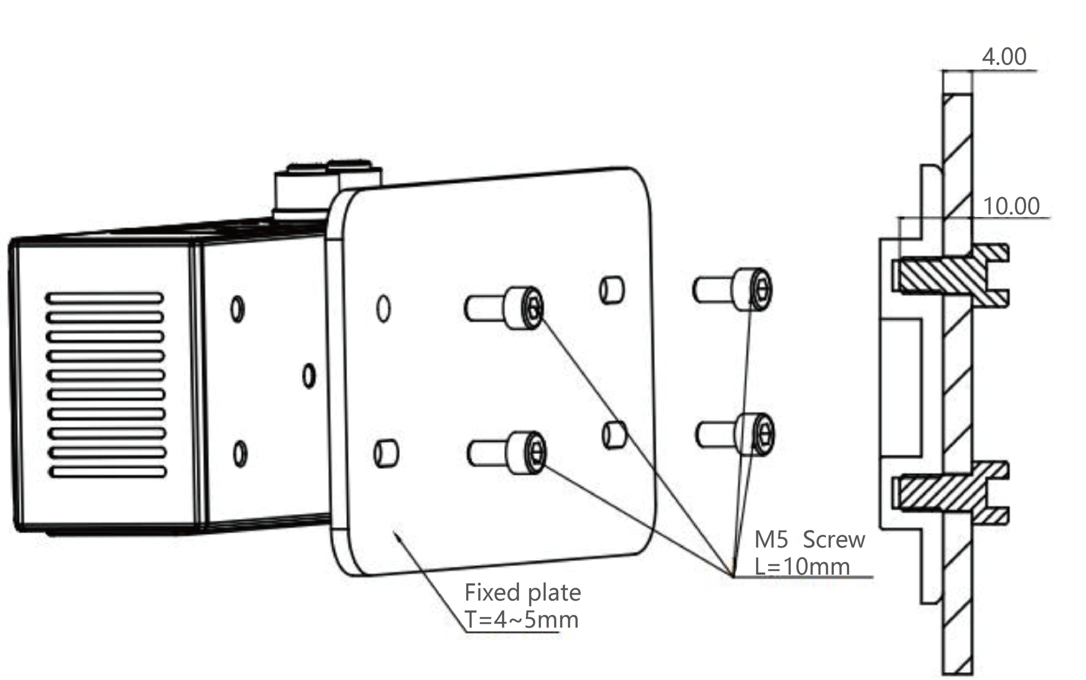
Figure 2.9 Camera installation diagram
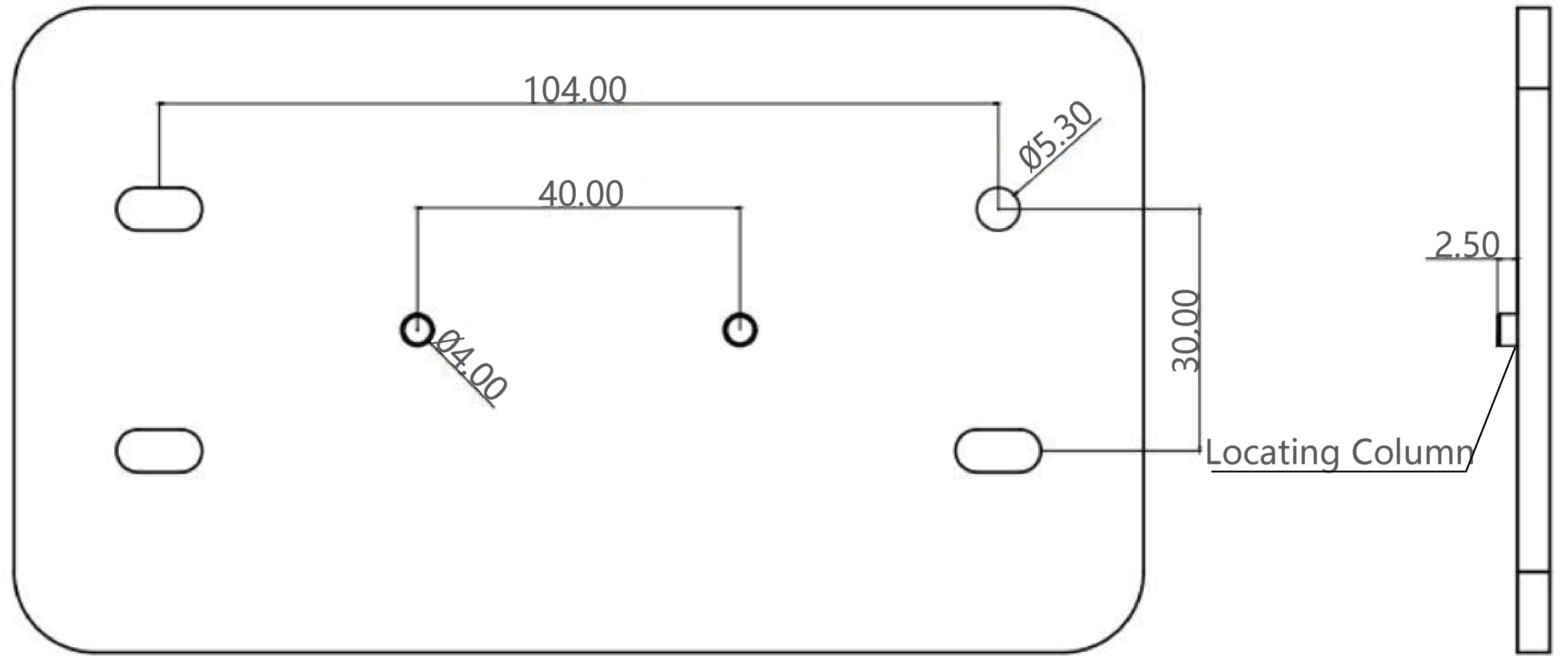
Figure 2.10 Recommended fixing plate size
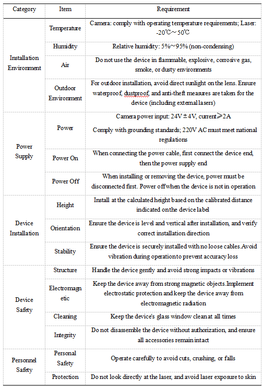
Installation Requirements:
Table 2-8 Installation Requirements
Usage Instructions and Precautions:
It is recommended to use the default resolution to reduce power-on initialization time and minimize time consumption.
If the camera disconnects unexpectedly, check whether the network cable and power cable are loose, ensure the software is running properly, or restart the camera.
Follow the instructions for proper operation, as improper handling may damage internal components.
Do not look directly into the projector after powering on to avoid eye discomfort.
Do not use other heat sources to heat the device.
Do not modify or disassemble the device in any way, as this may cause damage and reduce accuracy.
Avoid dropping or hitting the device to prevent internal component damage and accuracy degradation.
Do not touch the lens to avoid affecting image quality.
It is normal for the device to become warm after running for a period of time.
2.2. Equipment Installation
The camera and torch are mounted on the end of the robot via connectors as shown in Figure 2-11.
Important
Using the robot’s drag button as the reference point, the connecting piece is mounted directly behind it (passing radially through the center of the end flange to the opposite side).
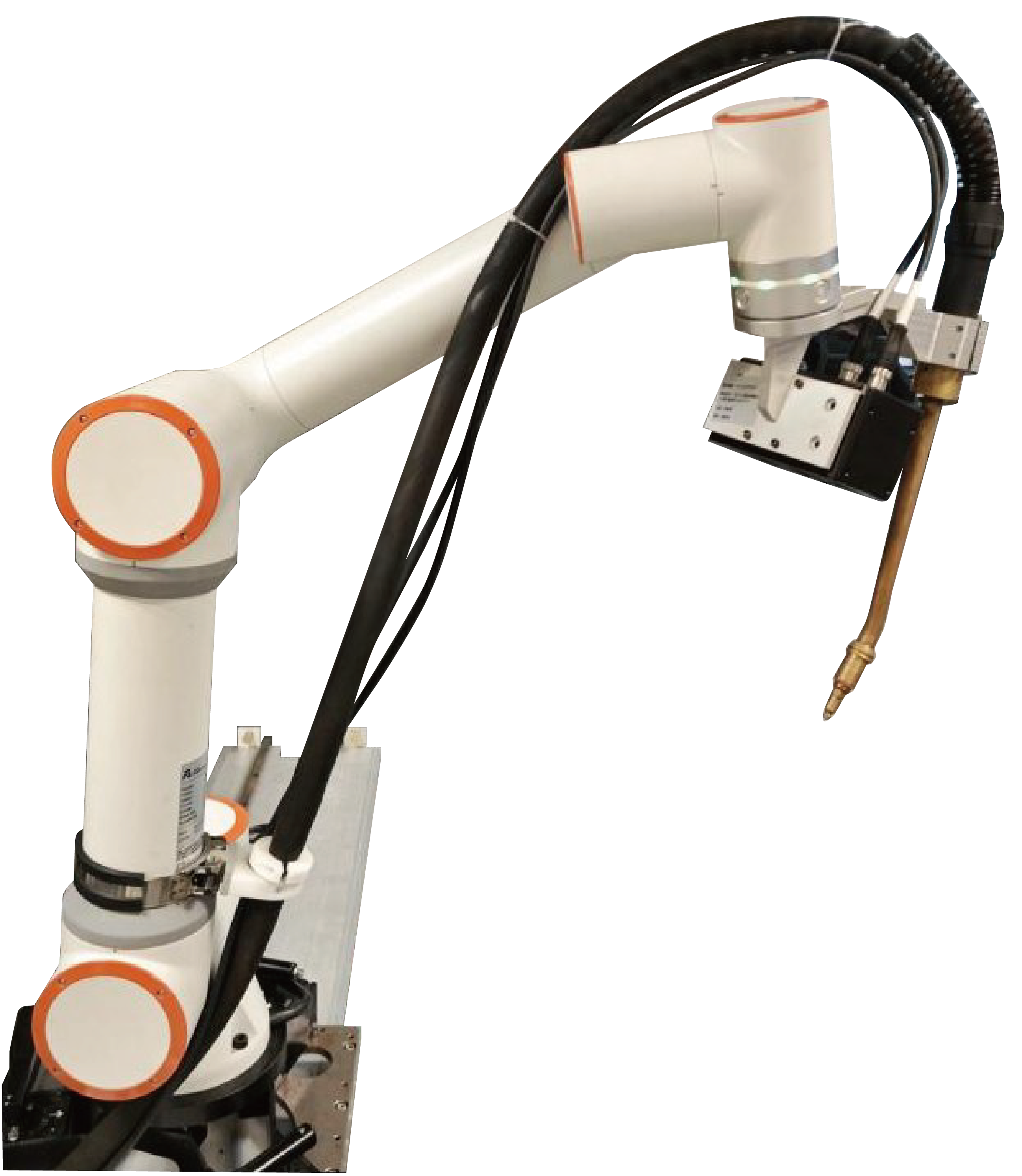
Figure 2.11 Mounting the Camera and Torch
Important
Please make sure to install it firmly, otherwise the accuracy will be affected.
2.3. Tool Coordinate System Calibration
AIRLab software provides a manual calibration function for the tool coordinate system. Import the robot and tool normally, click “Import Module” - “Tool” on the main interface, and open the tool settings interface(refer to Section 3.5.1). Then, select the tool coordinate system you want to calibrate and click the “Modify” button to enter the “Manual Tool Coordinate System Calibration” interface, as shown below.
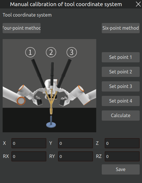
Figure 2.12 Manual Tool Coordinate System Calibration Interface
AIRLab offers two calibration methods: the Four-Point Method and the Six-Point Method. This document will introduce the Six-Point Method as an example. The detailed steps are as follows:
Important
Before calibration, confirm that the tool coordinate system, workpiece coordinate system, and extended axis coordinate system of the current application are all set to 0!
Step 1: Open the “Manual Tool Coordinate System Calibration” interface as mentioned earlier, then click the calibration method you want to use. In this demonstration, click the “Six-Point Method” button. The interface is shown below.
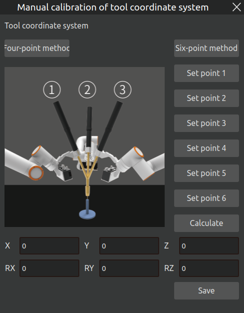
Figure 2.13 Calibration Method Setting
Step 2: Control the robot arm to align the end tool with the tip of the calibration tool (fixed reference point) in a certain posture. After the robot arm moves into position, click the “Set Point 1” button on the interface. When the button changes to “Modify Point 1”, the point is set successfully. To modify the set point, click “Modify Point 1” and repeat the steps. The process is shown in the figure below.
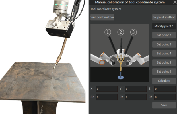
Figure 2.14 Setting Point 1
Step 3: Change the posture of the robot arm, again pointing the tool to the fixed reference point. After the robot arm moves into position, click the “Set Point 2” button. When the button changes to “Modify Point 2”, the point is successfully set. To change the point, click “Modify Point 2” and repeat the process. See the figure below.
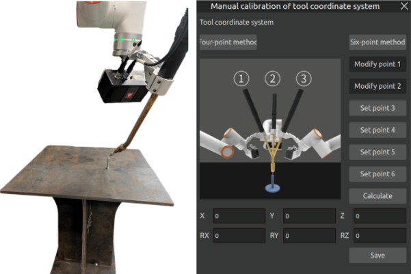
Figure 2.15 Setting Point 2
Step 4: Change the posture of the robot arm once again, pointing the tool to the fixed reference point. After the robot arm moves into position, click the “Set Point 3” button. When the button changes to “Modify Point 3”, the point is successfully set. To change the point, click “Modify Point 3” and repeat the process.After the setup of Point 3 is completed, the calibration point diagram on the page will switch to Point 4. Simply follow the diagram to start setting up Point 4. See the figure below.
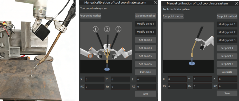
Figure 2.16 Setting Point 3
Step 5: Adjust the posture of the robot arm so that the tool end is vertically aligned with the fixed reference point, as shown in the left-side figure below. After the robot arm moves into position, click the “Set Point 4” button. When the button changes to “Modify Point 4”, the point is successfully set. To modify, click “Modify Point 4” and repeat the process. After the setup of Point 4 is completed, the calibration point diagram on the page will switch to Point 5. Simply follow the diagram to start setting up Point 5. See the figure below.
Important
When adjusting the posture of Point 4, the bent direction of the welding torch must be aligned with the X or Y axis direction of the robot base coordinate system! In this way, in Step 6, a single movement in the X or Y axis direction will yield Point 5.
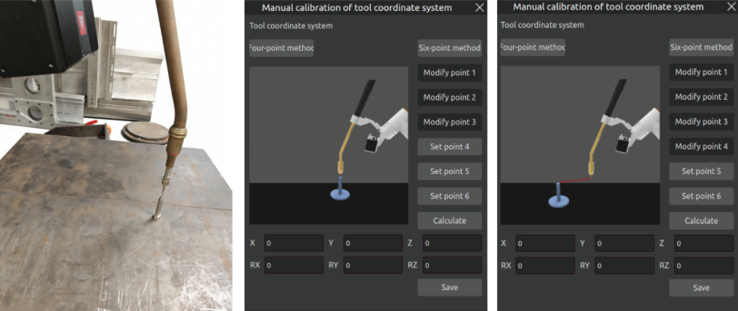
Figure 2.17 Setting Point 4
Step 6: Keep the robot arm’s posture unchanged, use base coordinate system movement to move a certain distance horizontally in the direction of the welding torch’s bend. This direction is the positive X-axis direction of the set tool coordinate system.. After the robot arm moves into position, click the “Set Point 5” button. When the button changes to “Modify Point 5”, the point is successfully set. To change, click “Modify Point 5” and repeat the process.After the setup of Point 5 is completed, the calibration point diagram on the page will switch to Point 6. Simply follow the diagram to start setting up Point 6. See the figure below.
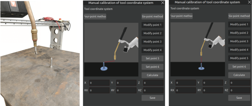
Figure 2.18 Setting Point 5
Step 7: Return to the fixed reference point and move vertically upward. This direction defines the positive Z-axis of the tool coordinate system. The positive Y-axis is determined according to the right-hand rule. After the robot arm moves into position, click the “Set Point 6” button. When the button changes to “Modify Point 6”, the point is successfully set. To modify, click “Modify Point 6” and repeat the process. See the figure below.
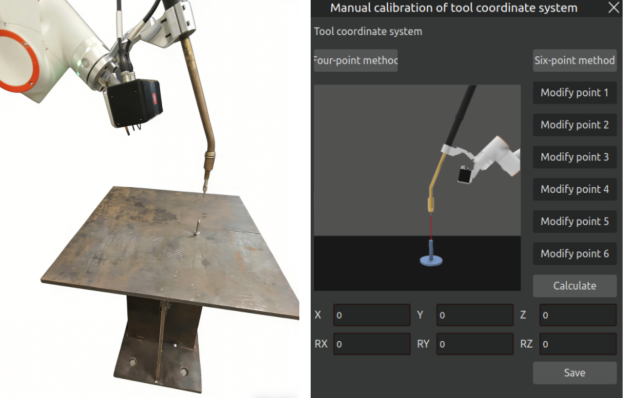
Figure 2.19 Setting Point 6
Step 8: After completing the above steps, click the “Calculate” button to compute the tool pose. The result is shown below.
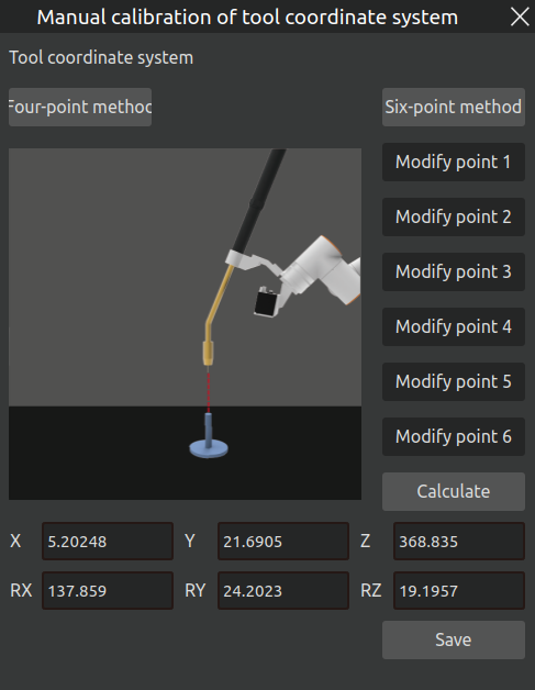
Figure 2.20 Tool Coordinate System Calculation Result
Step 9: After verifying the calculation result, click the “Save” button. The calibration result will be saved to the local path:~/AIRLabExe/Data/import_config/Cleargun_cutwire_settings.config under the section [Tool_coord_value_list]. In this example, tool3 is calibrated, so the saved entry will be:<3 = “calibration result”>At the same time, the calibrated tool3 option will also appear in the Tool Settings. See the figure below.
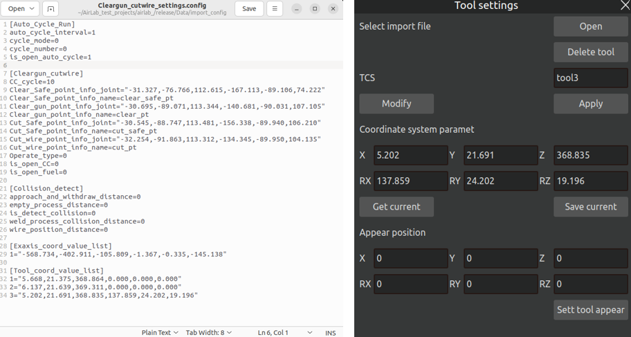
Figure 2.21 Saving Tool Coordinate System Result
If the selected tool coordinate system already exists (i.e., a value is already present under the above local path), a confirmation dialog will pop up asking whether to overwrite the previous result. If “Confirm” is selected, the previous result will be overwritten.
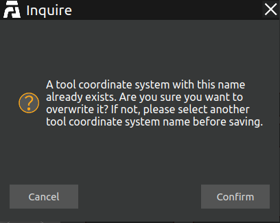
Figure 2.22 Tool Coordinate System Overwrite Confirmation Dialog
2.4. Point Cloud Camera Hand-Eye Calibration
After the robot is powered on, start the AIRLab software to ensure all modules are correctly initialized.
Step1: Camera connection
Open the camera module in the import module, and a “Camera Settings” pop-up window is displayed in the 3D scene.
Connect the camera; click Import Module -> Camera. The 3D scene displays the camera settings pop-up window, and the camera connects automatically. Upon successful connection, “Connection Status” in the pop-up window will display “Connected”, as shown in the figure below. If the connection fails, “Connection Status” will display “Disconnected”. In this case, please manually check whether the camera cable is connected correctly.
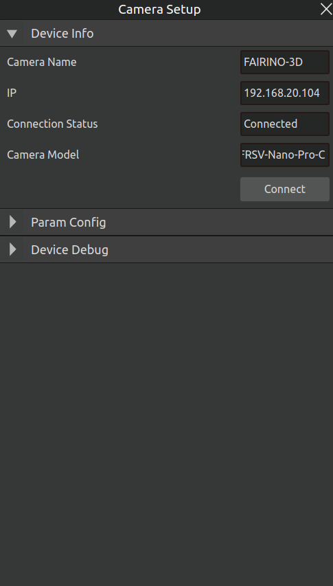
Figure 2.23 Camera Configuration - Search for Devices
Parameter configuration: Select the shooting mode as “Structured Light”, and set appropriate exposure time and other parameters as needed.
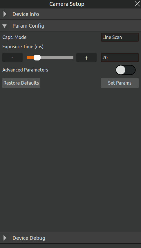
Figure 2.24 Set the shooting mode to “Structured Light”
Step2: Hand-Eye Calibration
Click on “Device Debugging” in the “Camera Settings” pop-up window. Then, click the “Hand-Eye Calibration” button, and a “Hand-Eye Calibration Pop-up” window will be displayed in the 3D scene, as shown in the figure.
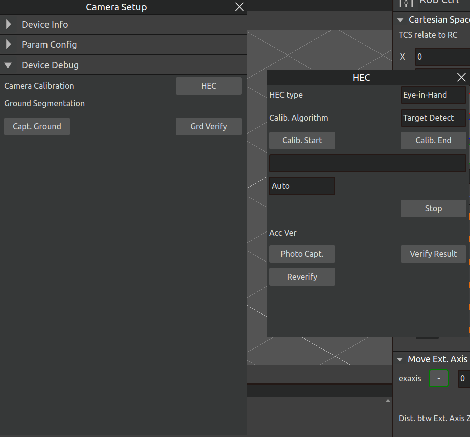
Figure 2.25 Hand-Eye Calibration Pop-up
Select the hand-eye calibration type and calibration algorithm, then click the “Calibration Start” button in the hand-eye calibration window to begin the calibration.
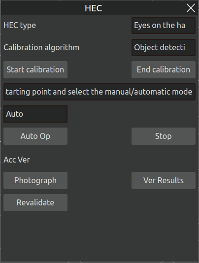
Figure 2.26 Calibration Start
Place the calibration board directly under the camera. The robot should control the end effector to position the camera directly facing the calibration board in a suitable posture, with the camera positioned at an effective shooting distance of 400–600 mm from the calibration board, as shown in Figure 2-24. Switch the main display area of AIRLab to the camera view, as shown in Figure 2-25.
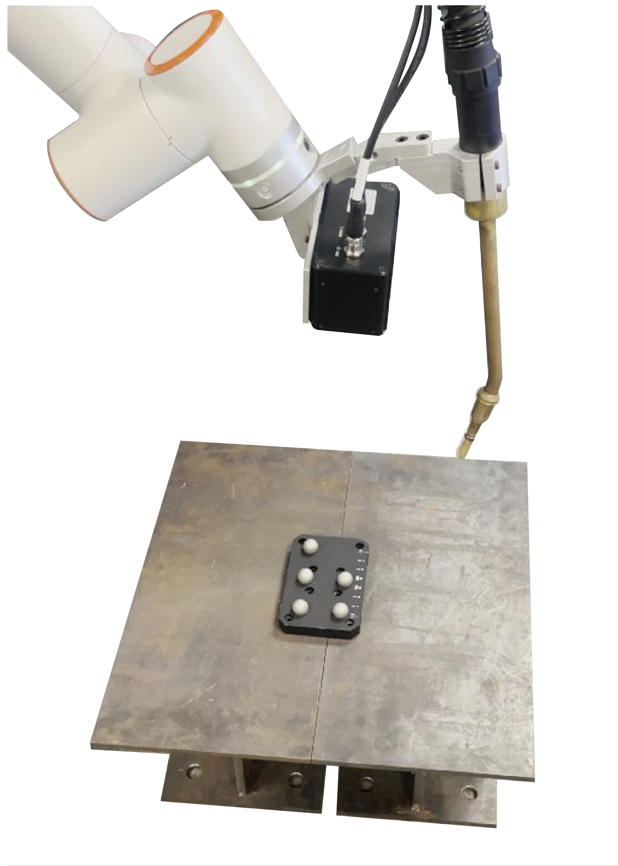
Figure 2.27 Placement of the calibration board
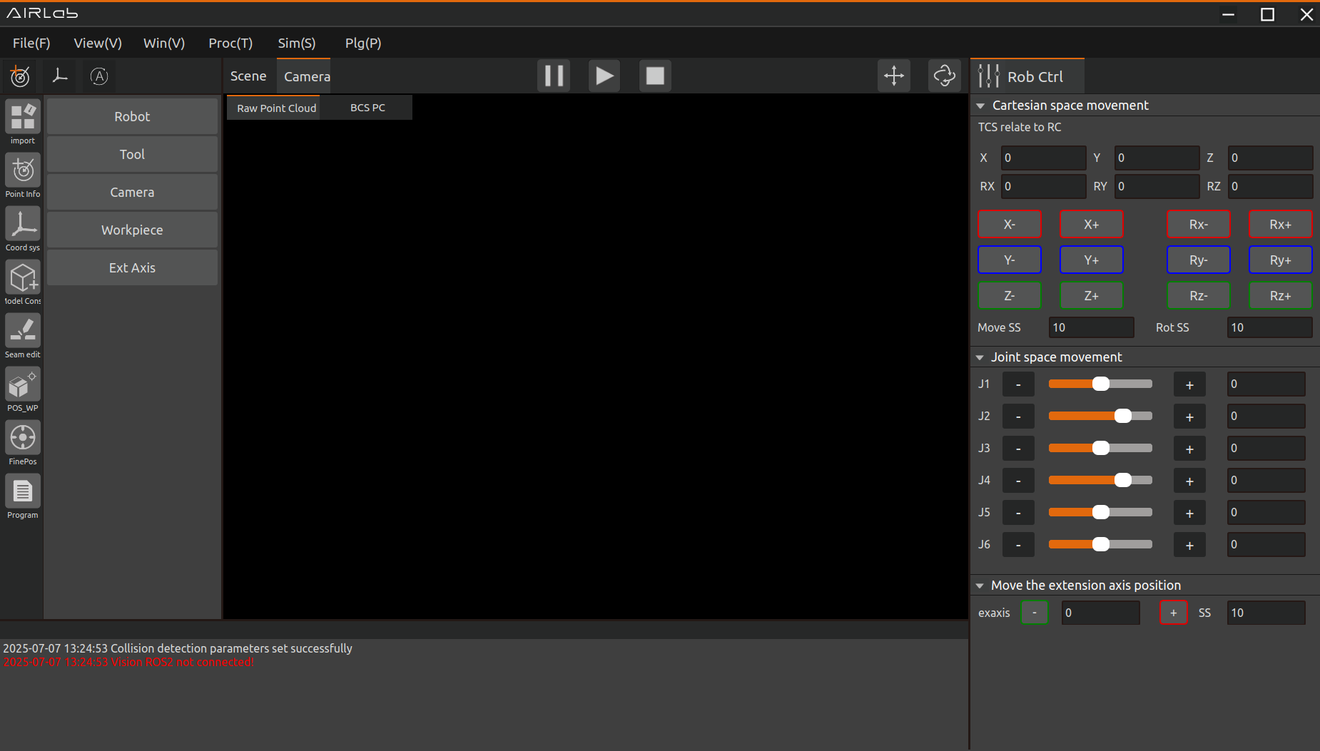
Figure 2.28 AIRLab Software-Camera Display
After selecting the operation mode as “Automatic,” click the “Auto Run” button. The software will then begin the hand-eye calibration automatically. During the image capture process, the camera will emit a blue light to indicate a successful shot. In automatic mode, the robot will autonomously capture images of the calibration board and change its pose accordingly. One complete cycle involves the robot altering its pose eight times and capturing eight images of the calibration board. If a calibration failure is prompted during the process, click the “Auto Run” button again to restart the current calibration cycle.
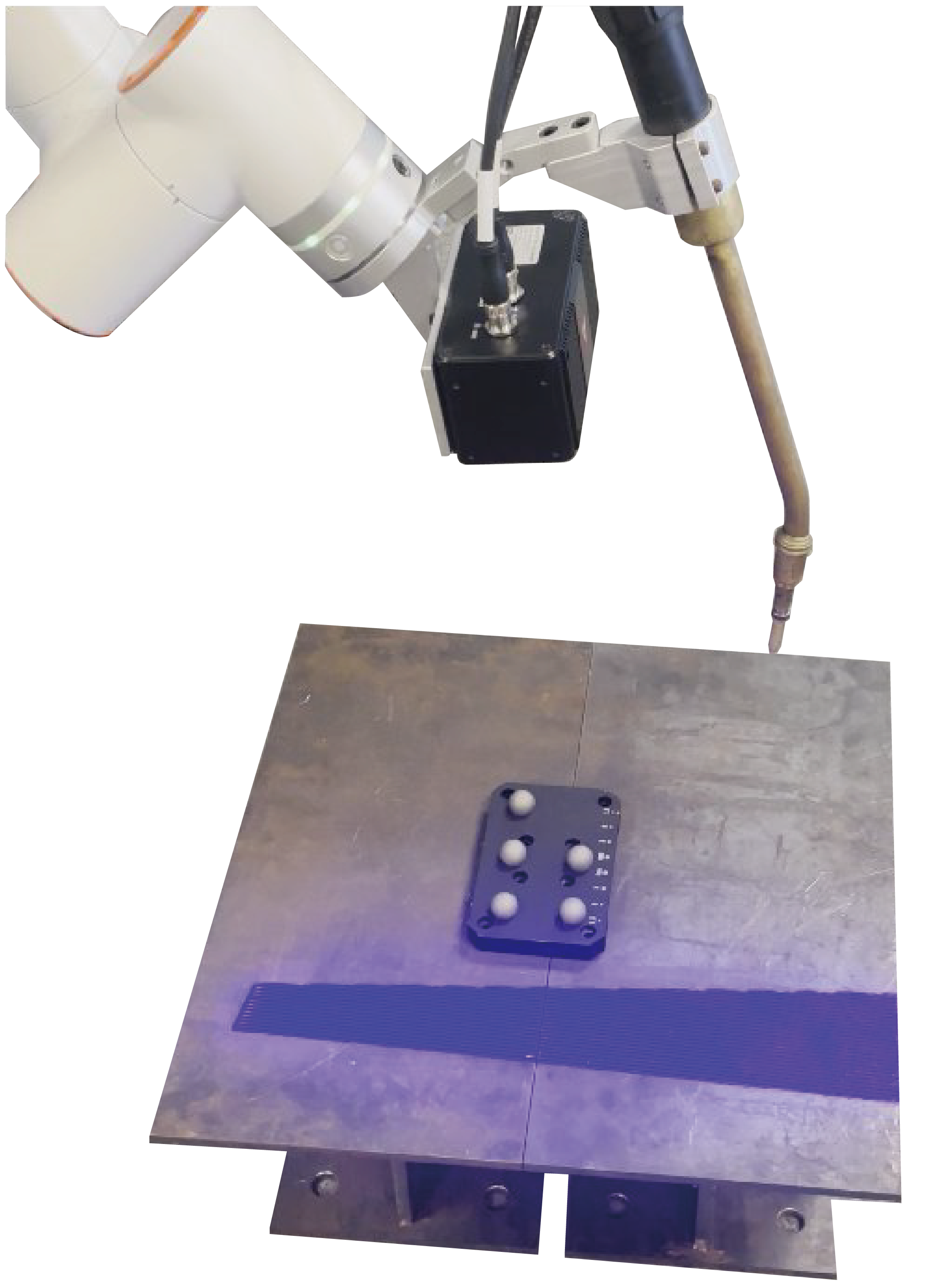
Figure 2.29 Point cloud camera hand-eye calibration
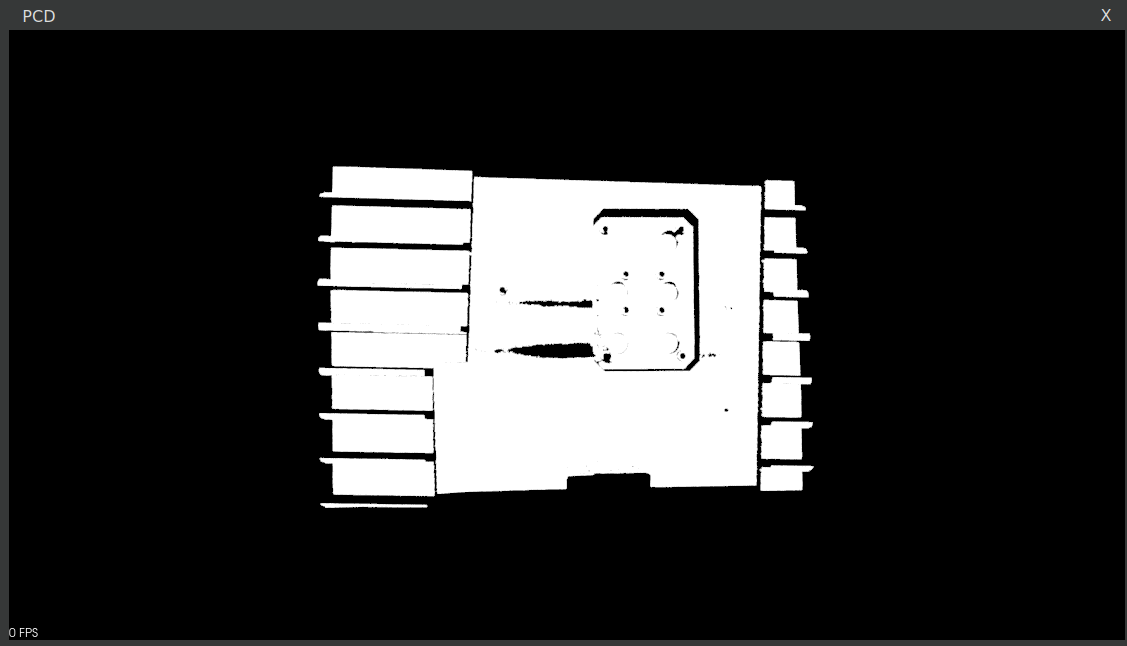
Figure 2.30 Point cloud calibration results
After the current round of camera calibration is completed, you can change the position of the calibration board and click the “Auto Run” button again to proceed with the next round of calibration. The purpose of this step is to improve system accuracy. You may choose to perform 3 to 5 rounds of calibration, and the system will automatically select the coordinate system with the highest accuracy for use.
After 3 to 5 rounds of calibration are completed, click the “Calibration End” button to finalize the hand-eye calibration of the camera.
Step3: Precision Verification
After the hand-eye calibration is completed, perform precision verification on the calibration results.
Manually drag the robot to position the camera directly facing the calibration board, ensuring the distance between the camera and the calibration board is between 400mm and 600mm. Click the “Re-verify” button to re-validate the hand-eye calibration results; then, click the “Capture” button under Precision Verification to take a photo. Upon successful capture, the software terminal will display a “Camera capture successful” message.
Manually drag the robot to change its posture. It is recommended to use eight postures in total: four with the forward joint configuration and four with the end joint reversed, as shown in the figure below. Each set of four postures should, as much as possible, cover the robot’s full range of joint motion. For each posture change, the interface difference must meet the following requirements: RX variation > 10°, RY variation > 10°, and RZ variation > 45°. Including the first photo taken for precision verification, a total of nine photos will be captured.
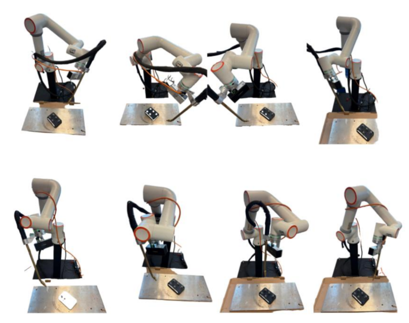
Figure 2.31 Accuracy Validation Pose Transformation
After successful accuracy verification shooting, click the “Verification Result” button. A pop-up window will appear showing “Error! Unrecognized switch parameter.” A comprehensive error value between 0.5mm and 1.0mm indicates that the hand-eye calibration result is good; a value between 1.0mm and 1.5mm indicates acceptable calibration results. Other results represent poor calibration, and recalibration is required.
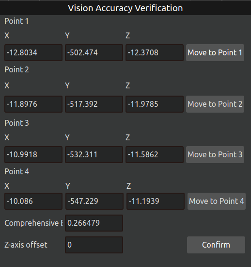
Figure 2.32 Authentication Results-Pop-up Window
If you need to re-verify, you need to click the “Revalidate” button to clear the error and then carry out the above verification process again. A combined error value in the range of 0.5 to 1.0 indicates a good hand-eye calibration result, while a value in the range of 1.0 to 1.5 indicates a lesser calibration result. Other results represent poor results for this calibration and require recalibration.
2.5. Ground Plane Acquisition and Verification
Before performing operational tasks for the first time, it is necessary to define the operational ground plane (if the operational ground plane is changed, this process must be repeated for re-confirmation). The operational steps are as follows:
Step 1: Open the “Camera Settings” interface, select “Structured Light” as the shooting mode, and click the “Device Debugging” header. Adjust the camera position to aim at the operational ground plane, then click the “Capture Ground” button to start ground capture.
Step 2: After completing ground capture, adjust the camera position to aim at the workpiece. Click the “Ground Effect Verification” button. The interface is shown in the figure below. Aim the camera at the workpiece and click the “Capture” button. After capturing, click the “View Segmented Point Cloud” button. The pop-up window will display the ground effect verification point cloud, as shown in the figure below.
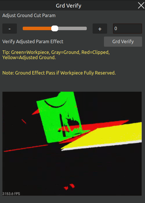
Figure 2.33 Ground Effect Verification Pop-up
In this display:The red point cloud represents the part of the workpiece that has been segmented (cut away) by the ground plane.The green point cloud represents the retained part of the workpiece.The gray point cloud represents the original ground plane.The yellow point cloud represents the ground plane adjusted with the new parameters.
If the verification result above does not meet expectations, you can adjust the ground segmentation parameters (by dragging the sliders or entering values in the text boxes). Click the “Ground Effect Verification” button at the bottom. The pop-up will then display the ground verification point cloud based on the new parameters, as shown below.
Check whether the point cloud from this ground verification meets the requirements (the ground plane is approximately flush with the bottom of the workpiece, and the workpiece is fully retained). If it meets the requirements, the ground effect verification is complete. Simply close the “Ground Effect Verification” pop-up window. If it does not meet the requirements, repeat the above steps of adjusting parameters, capturing, and viewing the segmented point cloud until the requirements are satisfied.
2.6. Model Reconstruction
Move the robot to teach the shooting points (the shooting range of the points should cover the workpiece model), and create a model reconstruction program, as shown in the figure below.
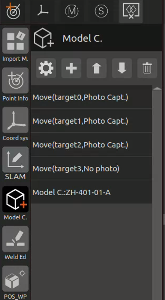
Figure 2.34 Model Reconstruction Program
Click “Run Program” as shown in the figure below. The robot will start moving, taking photos, and performing model reconstruction.
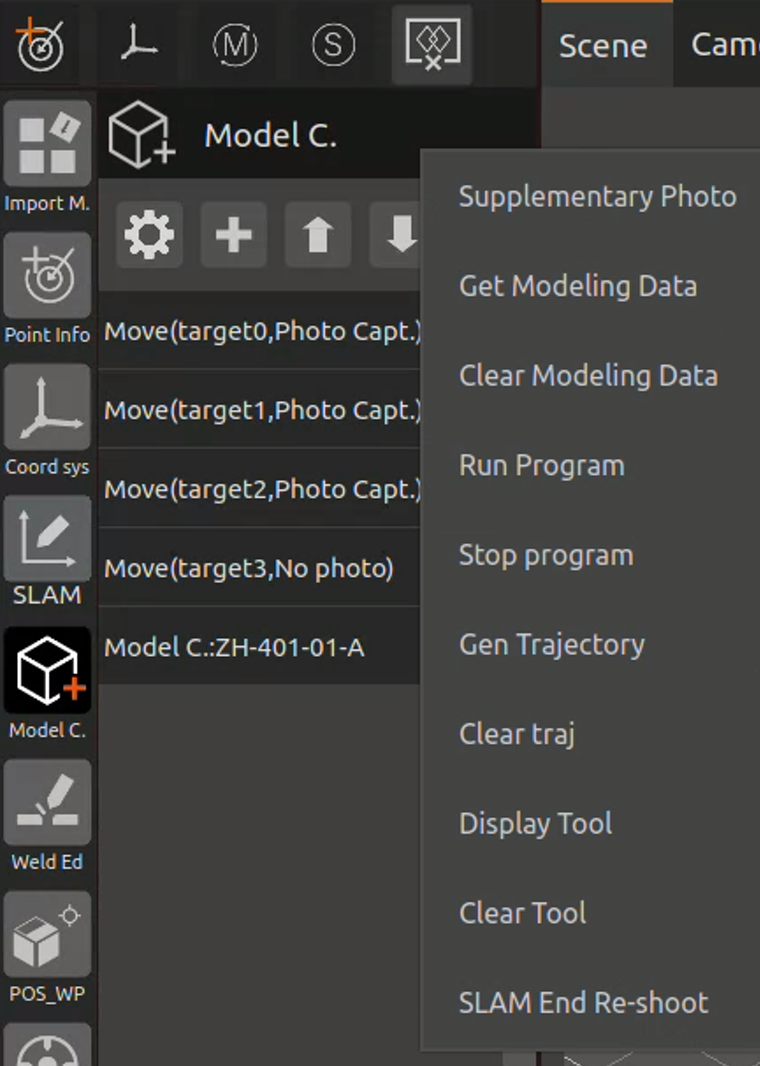
Figure 2.35 Model Reconstruction – Start Running
Upon successful reconstruction, the point cloud model of the workpiece will appear in the interface, as shown below.
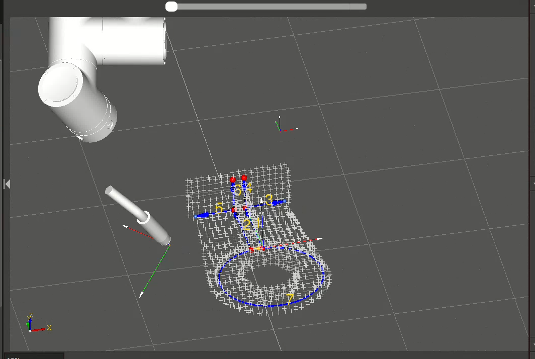
Figure 2.36 Successfully Reconstructed Workpiece Point Cloud Model
2.7. Start Running
After the model is successfully reconstructed, please complete the following steps in order: Weld Editing, Workpiece Positioning, and Fine Positioning Recognition. For detailed operation instructions, please refer to the Engineering Module analysis in Chapter 3 of this manual.
After the Lua program is successfully generated, please first set the parameters in the “Program Configuration” pop-up window, as shown in the figure below. For detailed parameter descriptions, please refer to the “Welding Program Configuration” section in Chapter 3 of this manual.
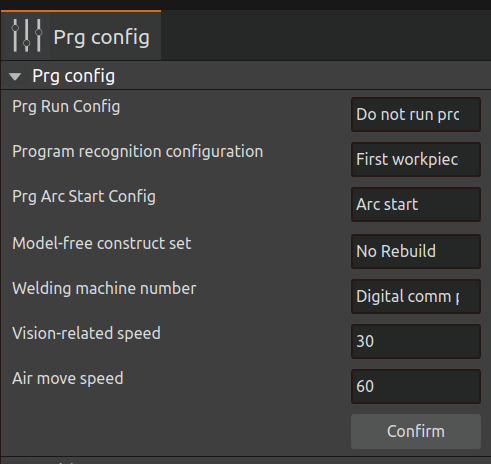
Figure 2.37 Setup Program Configuration
After configuration is complete, click “One-Click Run”. The program will start running from “Workpiece Positioning” until welding is completed.